"Before there were computers, there were algorithms." - H.Cormen. But now that there are computers, there are even more algorithms, and algorithms lie at the heart of computing. What are algorithms? Informally, an algorithm is any well-defined computational procedure that takes some value, or set of values, as input and produces some value, or set of values, as output. An algorithm is thus a sequence of computational steps that transform the input into the output. We can also view an algorithm as a tool for solving a well-specified computational problem. The statement of the problem specifies in general terms the desired input/output relationship. The algorithm describes a specific computational procedure for achieving that input/output relationship. For example, we might need to sort a sequence of numbers into nondecreasing order. This problem arises frequently in practice and provides fertile ground for introducing many standard design techniques and analysis tools.
This artilce is about algorithm theory introduction and just overview of algorithmic basics.
If computers were infinitely fast, any correct method for solving a problem would do. You would probably want your implementation to be within the bounds of good software engineering practice (for example, your implementation should be well designed and documented), but you would most often use whichever method was the easiest to implement. Of course, computers may be fast, but they are not infinitely fast. And memory may be inexpensive, but it is not free. Computing time is therefore a bounded resource, and so is space in memory. You should use these resources wisely, and algorithms that are efficient in terms of time or space will help you do so.
The complexity of an algorithm is the cost, measured in running time, or storage, or whatever units are relevant, of using the algorithm to solve one of those problems.
[6Ol2JbwoJp0]
Defining complexity classes
A complexity class is a set of problems of related complexity. Simpler complexity classes are defined by the following factors:
- The type of computational problem: The most commonly used problems are decision problems. However, complexity classes can be defined based on function problems, counting problems, optimization problems, promise problems, etc.
- The model of computation: The most common model of computation is the deterministic Turing machine, but many complexity classes are based on nondeterministic Turing machines, Boolean circuits, quantum Turing machines, monotone circuits, etc.
- The resource (or resources) that are being bounded and the bounds: These two properties are usually stated together, such as "polynomial time", "logarithmic space", "constant depth", etc.
To analyze an algorithm is to determine the amount of resources (such as time and storage) necessary to execute it. Most algorithms are designed to work with inputs of arbitrary length. Usually the efficiency or running time of an algorithm is stated as a function relating the input length to the number of steps (time complexity) or storage locations (space complexity).
Algorithm analysis is an important part of a broader computational complexity theory, which provides theoretical estimates for the resources needed by any algorithm which solves a given computational problem. These estimates provide an insight into reasonable directions of search for efficient algorithms.
Applications of complexity
Computational complexity theory is the study of the complexity of problems—that is, the difficulty of solving them. Problems can be classified by complexity class according to the time it takes for an algorithm—usually a computer program—to solve them as a function of the problem size. Some problems are difficult to solve, while others are easy. For example, some difficult problems need algorithms that take an exponential amount of time in terms of the size of the problem to solve. Take the travelling salesman problem, for example. It can be solved in time O(n22n) (where n is the size of the network to visit—let's say the number of cities the travelling salesman must visit exactly once). As the size of the network of cities grows, the time needed to find the route grows (more than) exponentially.
Big O notation
In mathematics, computer science, and related fields, big-O notation (also known as big Oh notation, big Omicron notation, Landau notation, Bachmann–Landau notation, and asymptotic notation) (along with the closely related big-Omega notation, big-Theta notation, and little o notation) describes the limiting behavior of a function when the argument tends towards a particular value or infinity, usually in terms of simpler functions. Big O notation characterizes functions according to their growth rates: different functions with the same growth rate may be represented using the same O notation.
[cVMKXKoGu_Y]
Summaries of popular sorting algorithms
Bubble sort - is a straightforward and simplistic method of sorting data that is used in computer science education. Bubble sort is based on the principle that an air bubble in water will rise displacing all the heavier water molecules in its way. The algorithm starts at the beginning of the data set. It compares the first two elements, and if the first is greater than the second, then it swaps them. It continues doing this for each pair of adjacent elements to the end of the data set. It then starts again with the first two elements, repeating until no swaps have occurred on the last pass. This algorithm is highly inefficient, and is rarely used, except as a simplistic example. For example, if we have 100 elements then the total number of comparisons will be 10000. A slightly better variant, cocktail sort, works by inverting the ordering criteria and the pass direction on alternating passes. The modified Bubble sort will stop 1 shorter each time through the loop, so the total number of comparisons for 100 elements will be 4950. Bubble sort may, however, be efficiently used on a list that is already sorted, except for a very small number of elements. For example, if only one element is not in order, bubble sort will only take 2n time. If two elements are not in order, bubble sort will only take at most 3n time. Bubble sort average case and worst case are both O(n²).
Selection sort - is a sorting algorithm, specifically an in-place comparison sort. It has O(n2) complexity, making it inefficient on large lists, and generally performs worse than the similar insertion sort. Selection sort is noted for its simplicity, and also has performance advantages over more complicated algorithms in certain situations. The algorithm finds the minimum value, swaps it with the value in the first position, and repeats these steps for the remainder of the list. It does no more than n swaps, and thus is useful where swapping is very expensive.
Insertion sort - is a simple sorting algorithm that is relatively efficient for small lists and mostly-sorted lists, and often is used as part of more sophisticated algorithms. It works by taking elements from the list one by one and inserting them in their correct position into a new sorted list. In arrays, the new list and the remaining elements can share the array's space, but insertion is expensive, requiring shifting all following elements over by one. Shell sort (see below) is a variant of insertion sort that is more efficient for larger lists.
Shell sort - was invented by Donald Shell in 1959. It improves upon bubble sort and insertion sort by moving out of order elements more than one position at a time. One implementation can be described as arranging the data sequence in a two-dimensional array and then sorting the columns of the array using insertion sort.
Comb sort - Comb sort is a relatively simplistic sorting algorithm originally designed by Wlodzimierz Dobosiewicz in 1980. Later it was rediscovered and popularized by Stephen Lacey and Richard Box with a Byte Magazine article published in April 1991. Comb sort improves on bubble sort, and rivals algorithms like Quicksort. The basic idea is to eliminate turtles, or small values near the end of the list, since in a bubble sort these slow the sorting down tremendously. (Rabbits, large values around the beginning of the list, do not pose a problem in bubble sort.).
Merge sort - takes advantage of the ease of merging already sorted lists into a new sorted list. It starts by comparing every two elements (i.e., 1 with 2, then 3 with 4...) and swapping them if the first should come after the second. It then merges each of the resulting lists of two into lists of four, then merges those lists of four, and so on; until at last two lists are merged into the final sorted list. Of the algorithms described here, this is the first that scales well to very large lists, because its worst-case running time is O(n log n). Merge sort has seen a relatively recent surge in popularity for practical implementations, being used for the standard sort routine in the programming languages.
Heapsort - is a much more efficient version of selection sort. It also works by determining the largest (or smallest) element of the list, placing that at the end (or beginning) of the list, then continuing with the rest of the list, but accomplishes this task efficiently by using a data structure called a heap, a special type of binary tree. Once the data list has been made into a heap, the root node is guaranteed to be the largest (or smallest) element. When it is removed and placed at the end of the list, the heap is rearranged so the largest element remaining moves to the root. Using the heap, finding the next largest element takes O(log n)O(n) for a linear scan as in simple selection sort. This allows Heapsort to run in O(n log n) time, and this is also the worst case complexity. time, instead of
Quicksort - is a divide and conquer algorithm which relies on a partition operation: to partition an array, we choose an element, called a pivot, move all smaller elements before the pivot, and move all greater elements after it. This can be done efficiently in linear time and in-place. We then recursively sort the lesser and greater sublists. Efficient implementations of quicksort (with in-place partitioning) are typically unstable sorts and somewhat complex, but are among the fastest sorting algorithms in practice. Together with its modest O(log n) space usage, this makes quicksort one of the most popular sorting algorithms, available in many standard libraries. The most complex issue in quicksort is choosing a good pivot element; consistently poor choices of pivots can result in drastically slower O(n²) performance, but if at each step we choose the median as the pivot then it works in O(n log n). Finding the median, however, is an O(n) operation on unsorted lists, and therefore exacts its own penalty.
Counting sort - is applicable when each input is known to belong to a particular set, S, of possibilities. The algorithm runs in O(|S| + n) time and O(|S|) memory where n is the length of the input. It works by creating an integer array of size |S| and using the ith bin to count the occurrences of the ith member of S in the input. Each input is then counted by incrementing the value of its corresponding bin. Afterward, the counting array is looped through to arrange all of the inputs in order. This sorting algorithm cannot often be used because S needs to be reasonably small for it to be efficient, but the algorithm is extremely fast and demonstrates great asymptotic behavior as n increases. It also can be modified to provide stable behavior.
Bucket sort - is a divide and conquer sorting algorithm that generalizes Counting sort by partitioning an array into a finite number of buckets. Each bucket is then sorted individually, either using a different sorting algorithm, or by recursively applying the bucket sorting algorithm. A variation of this method called the single buffered count sort is faster than quicksort and takes about the same time to run on any set of data.
Due to the fact that bucket sort must use a limited number of buckets it is best suited to be used on data sets of a limited scope. Bucket sort would be unsuitable for data such as social security numbers - which have a lot of variation.
Radix sort - is an algorithm that sorts numbers by processing individual digits. n numbers consisting of k digits each are sorted in O(n · k) time. Radix sort can either process digits of each number starting from the least significant digit (LSD) or the most significant digit (MSD). The LSD algorithm first sorts the list by the least significant digit while preserving their relative order using a stable sort. Then it sorts them by the next digit, and so on from the least significant to the most significant, ending up with a sorted list. While the LSD radix sort requires the use of a stable sort, the MSD radix sort algorithm does not (unless stable sorting is desired). In-place MSD radix sort is not stable. It is common for the counting sort algorithm to be used internally by the radix sort. Hybrid sorting approach, such as using insertion sort for small bins improves performance of radix sort significantly.
Distribution sort - refers to any sorting algorithm where data is distributed from its input to multiple intermediate structures which are then gathered and placed on the output. See Bucket sort.
Timsort - finds runs in the data, creates runs with insertion sort if necessary, and then uses merge sort to create the final sorted list. It has the same complexity (O(nlogn)) in the average and worst cases, but with pre-sorted data it goes down to O(n).
Sorting an array of a list of item is one of the base and most usefull data process. Here, we assume we have to sort an array (meaning we can access in constant time any item of the collection). Some of the algorithms we present can be used with other data-structures like linked lists, but we don't focus on this.
The most classical approach is called in-place, comparison based sorting. The sort visualizer presents only examples in this category. In place sorting means that, to save memory, one does not allow use of additional storage besides the items being compared or moved. Comparison-based sort means that we have a function (compare(a,b)) that can only tell if a<b, a>b or a=b. No other information on the keys is available, such as the ordinality of the items, nor is it possible to logically group them by any mean prior to sorting. Under such restrictions, any algorithm will require at least log n! (or O(n log n)) comparisons of one item again another to sort some array in the worst case. Any type of sort requires at least n moves in the worst case.
Non-comparison based sorts (radix sort, bucket sort, hash-tables-based, statistically based approaches...) assume that one can extract some ordinal information in the keys, and use it to improve the efficiency of the algorithm. For instance, to sort 100 integers, it is easier to group them by order of magnitude in one phase (0-9, 10-19...90-99...), then to sort the groups internally. Having more information on the key's range and structure allows to sort faster, often in linear time.
Sorts with additional buffers (merge sorts, quicksort (indirectly)...): Having a buffer to store intermediate results such as already sorted subportions of the array can help the efficiency of the algorithm, by reducing the number of moves that have to be performed. Nevertheless, it is not possible to go below the barrier of log n! comparisons in the worst case for comparison based sorts.
Algorithm Theory:
Algorithm theory deals with the design, analysis, and optimization of algorithms. An algorithm is a set of step-by-step procedures or a set of rules to be followed in calculations or problem-solving operations, typically by a computer. The primary goals of algorithm theory include:
- Correctness: Ensuring an algorithm correctly solves the problem it's designed to solve.
- Efficiency: Optimizing algorithms to use the least possible resources, typically time and space (memory).
- Simplicity: Designing algorithms that are simple and understandable.
Algorithm theory encompasses various strategies for developing algorithms, including divide and conquer, dynamic programming, greedy techniques, backtracking, and more. It also involves understanding different data structures that can efficiently support these algorithms.
Algorithm Complexity:
Algorithm complexity is a measure of the computational resources required by an algorithm to run. Complexity is usually expressed in terms of time (time complexity) and space (space complexity):
-
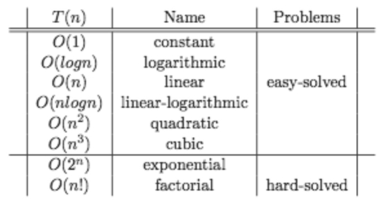
Time Complexity: Refers to the amount of time an algorithm takes to complete as a function of the length of the input. It is often expressed using Big O notation, which describes the upper bound of the time requirements in the worst-case scenario, e.g., O(n), O(n^2), O(log n).
-
Space Complexity: Refers to the amount of memory an algorithm needs to run to completion as a function of the length of the input. Like time complexity, it's often expressed using Big O notation, e.g., O(1), O(n), O(n^2).
Understanding algorithm complexity is crucial because:
- It helps predict the performance of algorithms in different contexts.
- It aids in identifying bottlenecks and optimizing resource use.
- It assists in choosing the most appropriate algorithm for a particular problem based on the available resources.
Classes of Problems in Algorithm Complexity:
-
P (Polynomial Time): Problems that can be solved in polynomial time, meaning the time required grows at a polynomial rate compared to the input size. For example, algorithms with complexities O(n), O(n^2) are considered efficient and are in class P.
-
NP (Nondeterministic Polynomial Time): Problems for which a solution, if given, can be verified in polynomial time, but it's not known whether these problems can be solved in polynomial time.
-
NP-Complete: A subset of NP problems that are as hard as the hardest problems in NP. If any NP-complete problem can be solved in polynomial time, all NP problems can be.
-
NP-Hard: Problems that are at least as hard as the hardest problems in NP. They might not even belong to the NP class (i.e., they might not be solvable via a deterministic Turing machine in polynomial time), but their solution is still critical for solving NP-complete problems.
Understanding these classes helps in evaluating the feasibility of algorithmic solutions for different problems and in researching new algorithms.
Conclusion:
Algorithm theory and complexity form the backbone of computer science, helping developers and theorists alike to design better algorithms, understand their limitations, and classify problems based on their solvability. They guide the development of software and systems that are more efficient, reliable, and scalable.
References
Algorithms
http://mitpress.mit.edu/instructors-manuals
AlgoComp.pdf (838.42 kb) from http://www.math.upenn.edu/~wilf/AlgComp3.html
Algorithmist, The -- dedicated to anything algorithms - from the practical realm, to the theoretical realm.
Algorithms Course Material on the Net
Algorithms in the Real World course by Guy E. Blelloch
Algorithmic Solutions (formerly LEDA Library) -- a library of the data types and algorithms ( number types and linear algebra, basic data types, dictionaries, graphs, geometry, graphics).
Analysis of Algorithms Lectures at Princeton -- Applets & Demos based on CLR.
Collected Algorithms(CALG) of the ACM
Complete Collection of Algorithm Animations (CCAA)
Data Structures And Number Systems -- by Brian Brown.
Function Calculator by Xiao Gang
FAQ - Com.graphics.algorithms -- maintained by Joseph O'Rourke
Game Theory Net
Grail Project -- A symbolic computation environment for finite-state machines, regular expressions, and finite languages.
Java Applets Center by R.Mukundan
Lecture Notes by Diane Cook
Lecture Notes for Graduate Algorithms by Samir Khuller
Maze classification and algorithms -- A short description of mazes and how to create them. Definition of different mazetypes and their algorithms.
Priority Queues -- Electronic bibliography on priority queues (heaps). Links to downloadable reports, researchers' home pages, and software.
Softpanorama Vitual Library /Algorithms
Ternary Search Trees -- Algorithm for search. PDF file and examples in C.
Traveling Salesman -- bibliography and software links.
MIT Video Lectures - Electrical Engineering and Computer Science > Introduction to Algorithms
Summary
Algorithms and they complexity is very cool and interesting topic for all developers. Because you and your programs need to be optimized in best way as you can. We want our ER doctors to understand anatomy, even if all she has to do is put the computerized defibrillator nodes on our chest and push the big red button, and we want programmers to know programming down to the CPU, algorithms and assembler level. What do you think about more articles about algorithms and best practices on them? Check out how different sorting algorithms sound like:
Sorting algorithms sounds:
15 Sorting Algorithms in 6 Minutes